MDPs & Reinforcement Learning
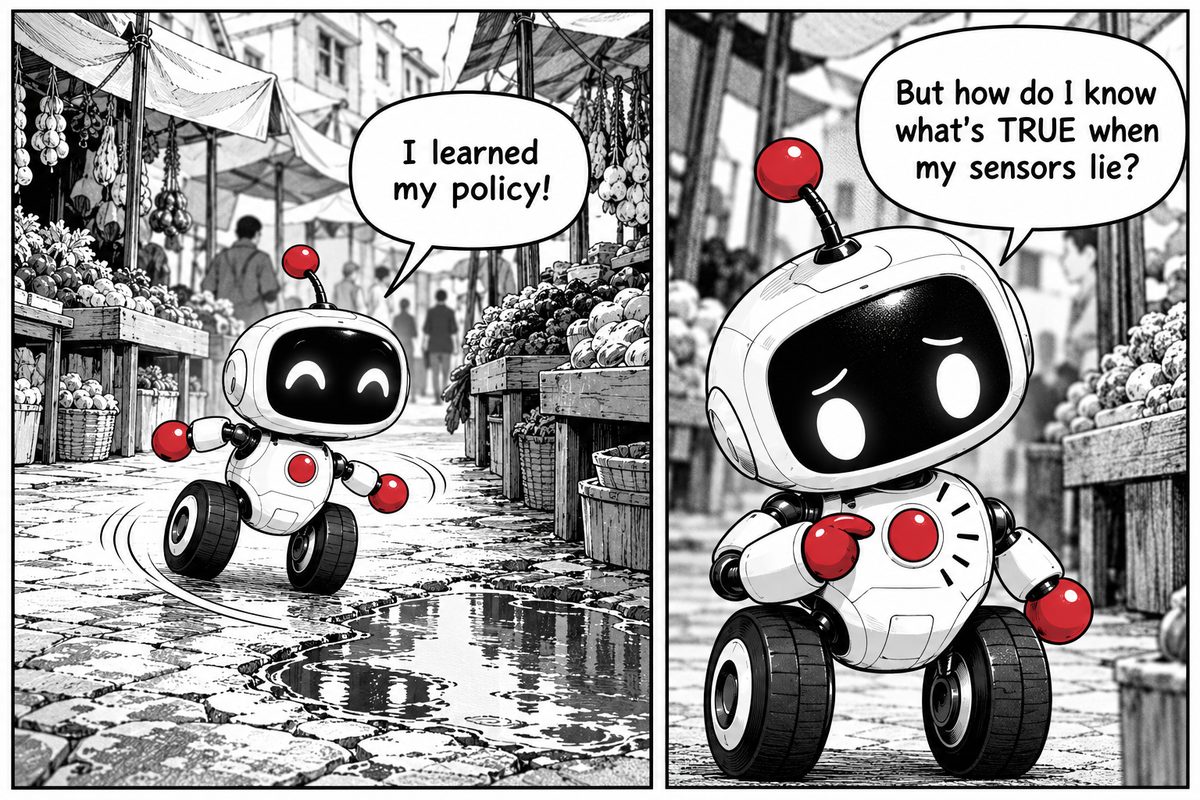
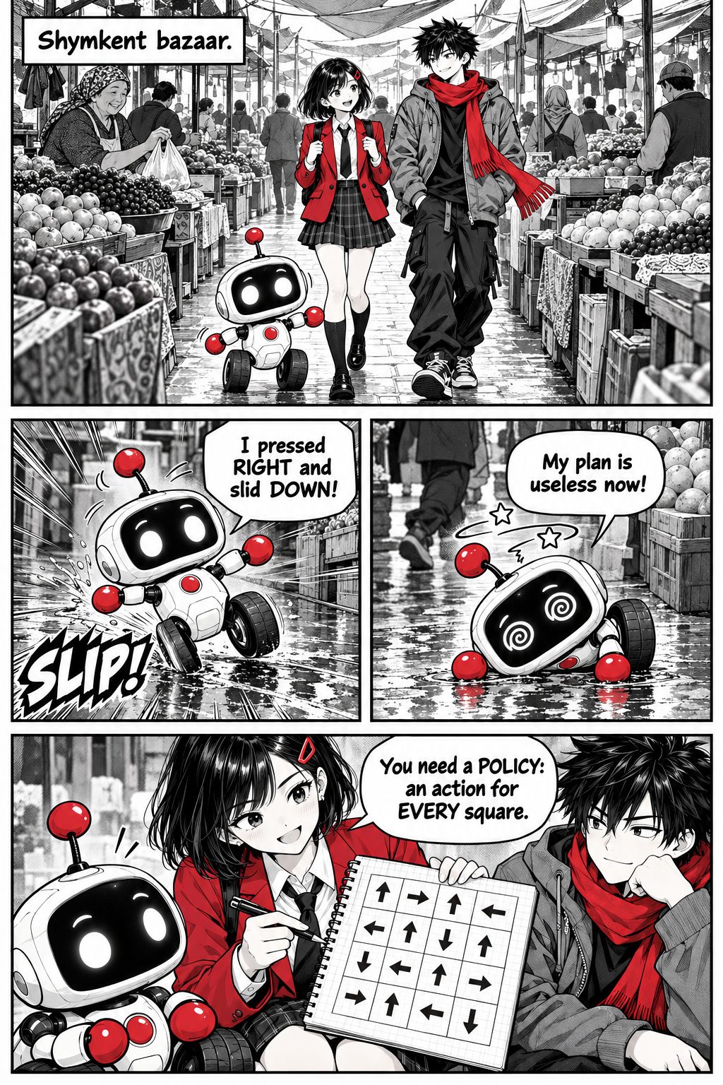
When the floor is slippery, a fixed path breaks. You need a policy: what to do in every state.
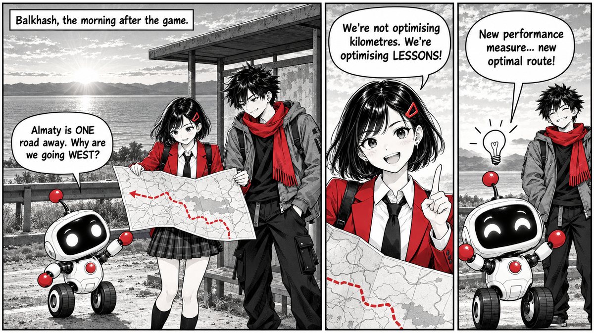
From Balkhash, Almaty is just one road away, yet Bota turns west to Shymkent, then north-east to Semey and Pavlodar, and only then south to Taldykorgan. Bota hasn't forgotten Chapter 2. Aru simply changed the performance measure (Chapter 1): the goal is no longer the cheapest road but the most lessons learned. Each city on the zigzag holds the next problem, so the "longest" route is the optimal one for this agent.
Sequential decisions under uncertainty
The action that looks best now can be bad in the long run. A machine that keeps running earns +10 per step but heats up; maintenance costs −15 now but prevents a −200 failure later. We optimise expected long-term return, not immediate reward.
Search returns a path (RIGHT, RIGHT, UP). If actions can fail, a path breaks. The solution to a Markov Decision Process (MDP) is a policy π(s): an action for every state.
The MDP model
- S: states (Bota's square; or a battery's charge, price and hour).
- A: actions (UP/DOWN/LEFT/RIGHT; CHARGE/HOLD/DISCHARGE).
- T(s′ | s, a): transition probabilities, e.g. RIGHT works 80%, slips UP 10%, DOWN 10%.
- R(s, a, s′): reward, e.g. goal +10, danger −10, each step −1.
- γ: discount factor, 0 ≤ γ ≤ 1.
Markov property: the next state depends only on the current state and action, not on the full history. The state must therefore contain everything that matters. A battery state with only "charge level" can't tell cheap hours from expensive ones, so price must be in the state.
Reward, return, value
A reward is immediate feedback. The return adds up future rewards with discounting:
| γ | 0.50 | 0.80 | 0.90 | 0.99 |
|---|---|---|---|---|
| Today's worth of a +100 reward 10 steps away (γ¹⁰·100) | ≈ 0.10 | ≈ 10.74 | ≈ 34.87 | ≈ 90.44 |
γ is a modelling choice about the effective horizon. For bounded rewards and γ < 1 it also keeps infinite-horizon returns finite; γ = 1 is safe only when episodes are guaranteed to end. Reward ≠ value: a square with reward 0 can be very valuable if it leads to +100 next. Value summarises the future.
The Bellman equation: now + later
Value = immediate reward + discounted value of where you land. Because the future after one step is again a decision problem, we can define values recursively:
Deterministic chain (lecture convention: the terminal GOAL state has a fixed value of 10): A → B → GOAL, step reward −1, γ = 0.9. V(B) = −1 + 0.9·10 = 8, V(A) = −1 + 0.9·8 = 6.2.
Stochastic example: RIGHT reaches GOOD (V=10) with 80% and BAD (V=−5) with 20%, step −1, γ = 0.9:
Q(s, RIGHT) = 0.8·[−1 + 0.9·10] + 0.2·[−1 + 0.9·(−5)] = 0.8·8 + 0.2·(−5.5) = 6.4 − 1.1 = 5.3.
Planning when the model is known
Value iteration repeats the Bellman update for all states until values stop changing. Goal information spreads backwards one step per sweep: on the 4-state chain, values go 0,0,0,10 → 0,0,8,10 → 0,6.2,8,10 → 4.58,6.2,8,10 (the lecture's simplified trace shows only states the goal has reached; applying the −1 step cost to every state gives −1,−1,8,10 → −1.9,6.2,8,10 → 4.58,6.2,8,10, with the same final values).
Policy iteration alternates policy evaluation (compute V^π) and policy improvement (in each state pick the action with the best one-step look-ahead) until the policy stops changing.
Each step costs −1. Fruit stall (goal) = +10, spilled oil (pit) = −10, both terminal. Moves succeed with 80% probability and slip sideways 10% each way. Bumping into a wall or the edge means staying put.
Sweep 0: all values start at 0. Arrows show the greedy policy.
Raise slip to 40–60%. Next to the pit, the policy starts walking away from the danger even though the route gets longer. Lower γ to 0.3 and the far squares barely care about the goal: their values stay close to the step cost.
Reinforcement learning: when the model is unknown
Real systems rarely tell us T and R exactly. What is P(failure tomorrow | vibration = 6.5, load = 92%)? Reinforcement learning (RL) learns a good policy from experience (s, a, r, s′) gathered by interacting with the environment or a simulator.
| Supervised learning | Reinforcement learning | |
|---|---|---|
| Feedback | The correct label for each input | A reward, often delayed; nobody says which action was "correct" |
| Data | Fixed dataset, samples treated as independent | The agent's own actions decide what data it sees next |
Exploration vs exploitation: exploit what looks best now, or explore to discover something better? ε-greedy: with probability ε take a random action, otherwise the best known one (ε = 0.1 means about 10% exploration).
Learning from surprise: temporal difference
Monte Carlo methods wait for the episode to end and use the actual return. TD methods update after every step by bootstrapping: they use their own estimate of the next state.
Q-learning
Worked update: Q(A, RIGHT) = 4, r = 2, max Q(B,·) = 8, γ = 0.9, α = 0.5. Target = 2 + 0.9·8 = 9.2, error = 5.2, new Q = 4 + 0.5·5.2 = 6.6.
Three parameters, three different jobs: α sets how strongly one experience changes the estimate, γ sets how much the future matters, ε sets how often to explore. Q-learning is off-policy: its target uses max Q, the greedy action. SARSA is on-policy: it uses the action actually taken next, Q(s′, a′).
States 0–4, actions LEFT/RIGHT, step reward −1, reaching state 4 gives +10. The Q-table starts at all zeros: Bota knows nothing.
Episodes trained: 0
Scaling up: deep RL
Tables don't scale. A battery with 10 charge levels × 20 prices × 20 demand levels × 20 solar levels × 24 hours already has 1,920,000 states, and 5,760,000 Q-values with 3 actions. Deep Q-Networks (DQN) approximate Q(s, a; θ) with a neural network, stabilised with replay buffers and target networks. Policy-gradient methods learn πθ(a|s) directly, which suits continuous actions. Actor–critic methods combine both: the actor chooses, the critic evaluates.
A high reward is not permission to break engineering limits. Badly designed rewards get "hacked": the agent optimises the number, not the real goal. Real deployments train in simulators first, encode hard safety constraints separately and keep human override.
RL controls data-centre cooling, battery charging, robot locomotion and game agents (AlphaGo, Atari-playing DQN). Language models are also fine-tuned with RL from human feedback (Chapter 10).
1. Why can a state with reward 0 have high value?
2. Which parameter controls how often the agent tries random actions?
3. Q(s,a)=4, r=2, max Q(s′)=8, γ=0.9, α=0.5. New Q?